The math of risk equalization

June 27th, 2023

Piet Stam

Meet & greet

• What do you expect to learn from this course?
• My agenda
  • First, an intro to the math
  • Second, applying it to some data
• R package rvedata based on my PhD thesis

Context

• 🇳🇱 health care (basic benefits)
• 🇳🇱 health insurance
• 🇳🇱 system of risk equalization
• Traditional focus on incentives
  • NOT actual behavior
  • NOT effects (efficiency & equity)

Data collection

• Large national data set
• Population vs. sample
• Weights for insurance period
• Multiple records per insured
• Pseudonyms for merging data sets

Which are the “acceptable costs”?

“The costs of services that follow from a quality, intensity and price level of treatment that the sponsor considers to be acceptable to be subsidized.” (Van de Ven and Ellis, 2000)

• Two extremes:

  • Best practice costs
  • Actual expenditures

• Q: which is more health based?

• 🇳🇱: Y = actual expenditures with average prices for some services

• Q: with this definition, is Y health based?
• A: no, it is production based
• I: therefore, compensation can hardly be made health-based

Which subgroups to compensate?

“The REF equation should only include parameters which equalize cost differences in health status of an insured as a consequence of differences in age, gender and other objective measures of health status.” (Health Insurance Decree:389, p.23)

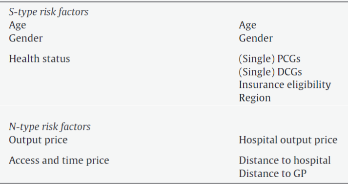
Compensation for S(olidarity)-type groups

• Age
• Gender
• Health status

No compensation for
N(on-solidarity)-type groups

• Propensity to consume
• Input prices
• Regional overcapacity (SID)
• Provider practice style

The regression equation

\[ \begin{aligned} Y &= f(S,N) + u \\ &= S \alpha + N \gamma + u \\ &= \sum_{l=1}^L S_l \alpha_l + \sum_{m=1}^M N_m \gamma_m + u \end{aligned} \]

with

• \(Y\) health expenses observed during some period in time
• \(S_l\) is the \(l\)th S-type risk factor, \(l=1,...,L\)
• \(N_m\) is the \(m\)th N-type risk factor, \(m=1,...,M\)
• (\(u \sim IID(0,1)\))

• Q: why IID condition between brackets?
• A: because it is not needed to apply OLS
• I: it is only needed if you need standard errors

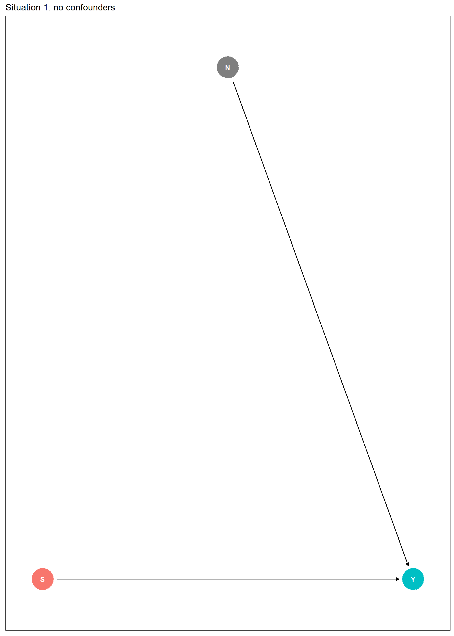
Which causal diagram?

Situation 1: more supply (N) -> more Y Situation 2: more supply (N) -> more Y, better health Situation 2: too much supply (N) -> worse health b/o over treatment Situation 3: sick people (H) -> move to more/better supply in big cities (N)

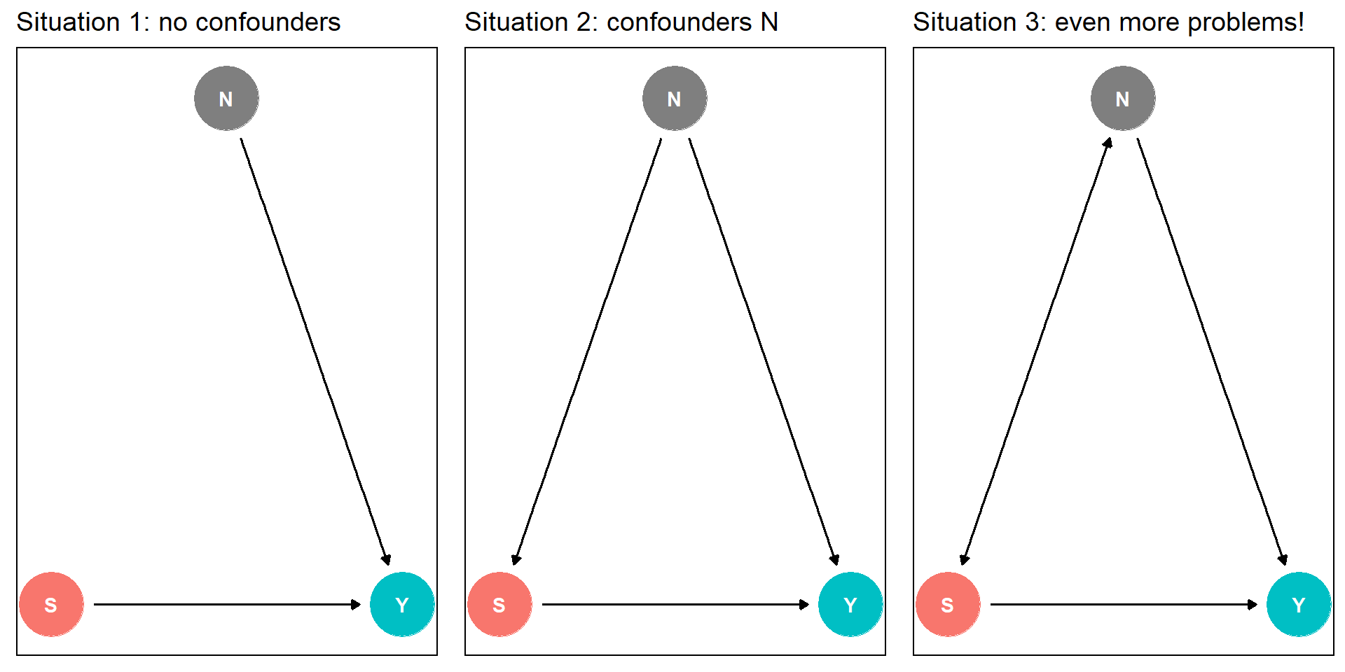
Big assumption

Define \(v := N \gamma + u\) and rewrite \[ \begin{aligned} Y &= S \alpha + N \gamma + u \iff \\ Y &= S \alpha + v \end{aligned} \]

\[ \begin{aligned} \implies \hat{\alpha} &= (S'S)^{-1}S'Y \\ &= (S'S)^{-1}S'(S \alpha + v) \\ &= \alpha + (S'S)^{-1}S'N\gamma + (S'S)^{-1}S'u \end{aligned} \]

\[ \implies E[\hat{\alpha} | S,N ] = \alpha \iff \begin{aligned} \begin{cases} S'N = 0 \\ \gamma = 0 \end{cases} \end{aligned} \]

What to do if assumption fails?

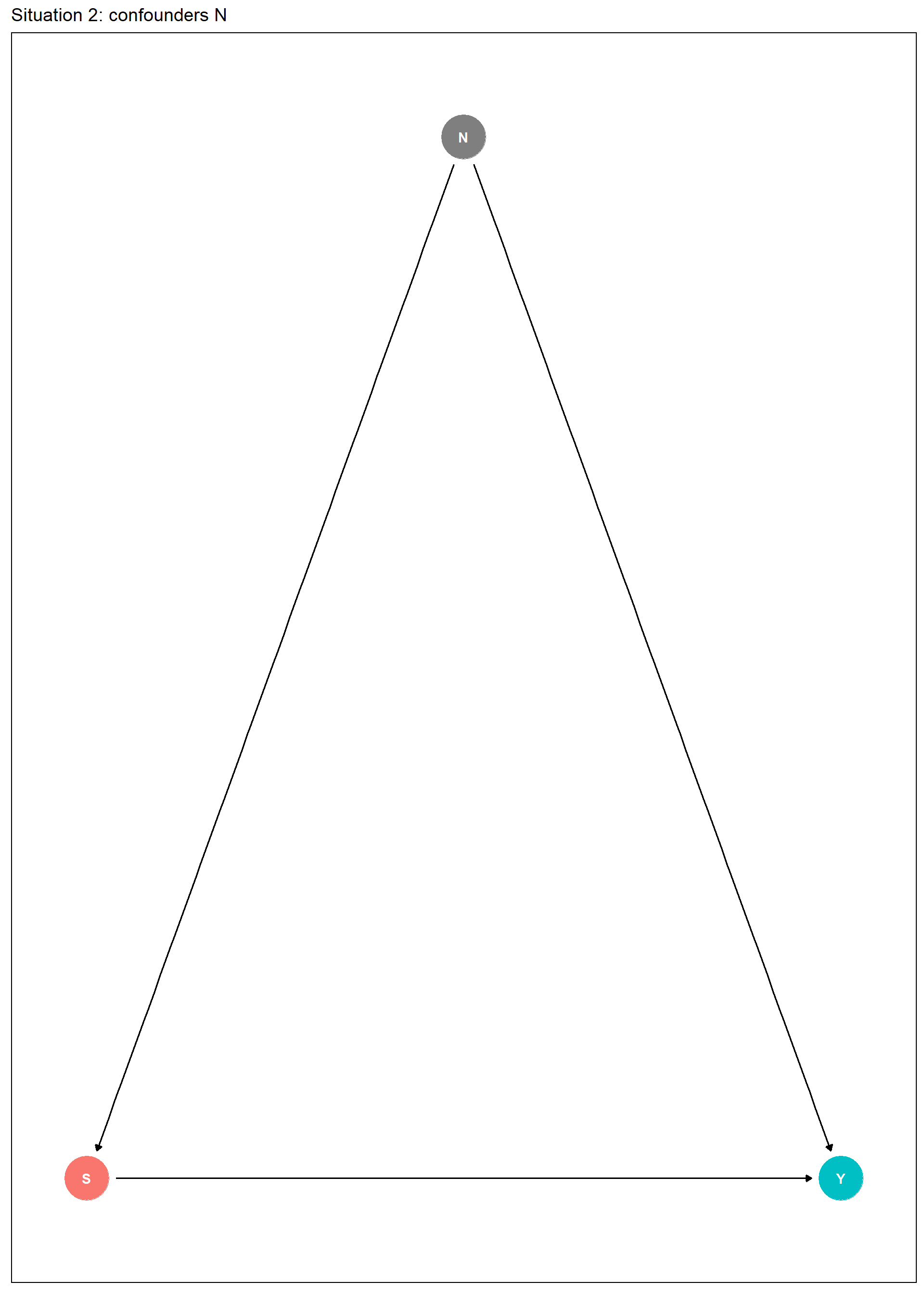
Schokkaert and Van de Voorde () recommend a 2-step method:

1. estimate (\(\alpha, \gamma)\) in regression with \(S\) and \(N\) variables
2. predict \(Y\) with \(N\) set at prevalences

The formula then reads as follows:

\[ \hat{Y} = S \hat{\alpha} + \overline{N} \hat{\gamma} \] with \(\overline{N}\) being a row i/o matrix.

Or… ignore this omitted vars bias

In practice, we apply this equation:

\[Y = X \beta + \epsilon\]

and try to extend \(X\) with as much (measurable) S-type variables as possible.

Regression without an intercept

Traditional OLS:

• include an intercept
• omit one category of age/gender
• omit one category of each other \(X\) (which one?)

OLS w/ risk equalization:

• do not include an intercept
• include all categories of all other \(X\)’s
• set total effect of age/gender := sum of \(Y\)
• set total effect of each other \(X\) := 0

Apply weights

• Weights \(W\) define length of insurance contract
• \(0 < W <= 1\)
• Potential reasons for \(W < 1\):
  • 2 or more records for 1 individual -> sum Y and X
  • babies born
  • people deceased

Use aggregation to save computer time

• “Vertical aggregation” for each unique combination of X
• Total number of rows = number of unique combinations
• W := sum of observations for each unique combination
• Y := average expenses \(\overline{Y}\) for each unique combination
• X := set of prevalences \(\overline{X}\) for each unique combination
• OLS estimation using these W, Y and X
• Bekijk mijn blog voor een eenvoudig voorbeeld

Region: individual & zip code data

• In 2002 a two-step approach was implemented:
  • step 1: \(Y = X \beta + \epsilon\) (indiv. level)
  • step 2: \(\epsilon = Z*c + \xi\) (zip-code level)
• As \(\hat{\epsilon} = Y - \hat{Y}\) step 2 can be read as:
  • step 2: \(Y = 1.\hat{Y} + Z*c + \xi\)
• Implicit restriction: \(\hat{Y}\) and \(Z\) not correlated
• If this assumption is false, the estimators are inconsistent
• Therefore, \(\hat{Y}\) was added to step 2 since the 2006 model
• Nowadays, one comprehensive regression at indiv. level

(Ex post) risk sharing

Definition: insurers are retrospectively reimbursed for some of the costs of some of their insurance members (Van de Ven and Ellis 2000)

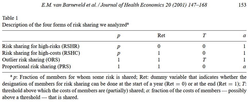
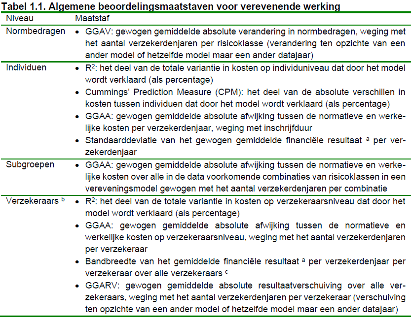
Assessment framework

Install package rvedata

• Source: https://github.com/risicoverevening/rvedata

• Metadata rvedata

https://pietstam.nl/talks